iDQ online
What does this task do?
This task queries iDQ results from the independent, asynchronous runs managed outside the DQR. In order to expedite the availability of results, the query is broken into several pieces.
a rapid query that only examines a small window around the candidate. This window is determined by the properties of the candidate, like the template duration, as defined within the DQR (see
idq.gracedb.graceid2start_end()). This includes the following, which will all be rendered within the DQR HTML interfacetimeseries for the duration of the small window
calibration distributions for all CalibrationMaps used to generate timeseries within the small window
feature importance figures and tables for all ClassifierModels used to generate timeseries within the small window.
Please note, the precise nature of the feature importance information will depend on which classifier is available.
a broader query to estimate iDQ’s local performance with larger sample sizes. The broader query is summarized in a separate HTML document, which is linked from the DQR interface. This separate document is will include
an overview/comparison page with
timeseries within the small window
Receiver Operating Characteristic curves for all samples within the broader query
all calibration distributions used within the broader query
calibration coverage plots for all samples available within the broader query
feature importance figures and tables for the broader query (if available)
correlations between multiple classifiers for all samples witin the broader query (if available)
single-classifier summary pages with
timeseries within the broader query
calibration coverage and distributions for each CalibrationMap separately
feature importance tables and figures as well as Receiver Operating Characteristic curves for each ClassifierModel separately.
It is worth noting that iDQ online jobs only summarize information already generated asynchronously. They do not generate any new information or measure any auxiliary couplings themselves, unlike iDQ offline and pointy-poisson jobs.
What are its return states?
human_input_needed
error
How was it reviewed?
This has not been reviewed!
How should results be interpreted?
iDQ provides many different types of information to measure the ability to predict the presence of glitches in a target channel (typically a proxy for h(t)$) and auxiliary channels. Although a full description of iDQ’s methodology is outside the scope of these documents (see the [iDQ source documentation](https://docs.ligo.org/reed.essick/iDQ/) instead), we briefly describe the main data products presented in these summaries. Some of this information is included in the rapid initial query over a small window and will be rendered within the DQR HTML interface, but analysts should expect to click through to the full iDQ summary reports as well.
Within the DQR HTML Interface
In addition to rendering a few key pieces of information (see below), the DQR HTML interface will render the following links.
iDQ online DQR documentation (this page)
and when the full summary report is available, there will also be a link to it. That link is included in the summary and in the links section.
Basic Statitics
Several basic statistics are presented within the DQR. The header includes inforamtion about the fraction of time within the small window with p(glitch|aux) above a threshold. p(glitch|aux) can be thought of as the ultimate produce produced by iDQ, and represents the probability of a non-Gaussian noise transient being present within h(t) given the information in the auxiliary channels. This header additionally changes when the final summary becomes available. Before the summary is available, the header will resemble the following
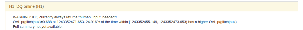
and after the broader summary is available, it will change to
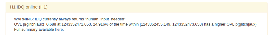
There are a few other statistics reported in the DQR HTML interface, associated with the particular classifiers summarized. An example is below

Because the online reports represent queries to asynchronous processes that continuously update, there may be more than one ClassifierModel or CalibrationMap associated with the small query. These objects are used to map the auxiliary state of the detector into statistical predictions about the presence of a glitch, and as they are updated the predictions may change. Therefore, the DQR reports the number of CalibrationMaps and ClassifierModels used to produce the timeseries output within the small window. It also reports iDQ’s duty cycles with respect to wall-time and science time within the small query (i.e., whether any data was missing).
Timeseries
iDQ produces various types of timeseries as output. The DQR summarizes several of these within the small query window surroudning the event. An example figure is below. Analysts should examine the figure and look for excursions within the timeseries that suggest the presence of non-Gaussian noise. However, the presence of non-Gaussian noise does not necessarily mean the candidate should be rejected and care must be taken to determine whether the non-Gaussian noise could have caused the candidate.
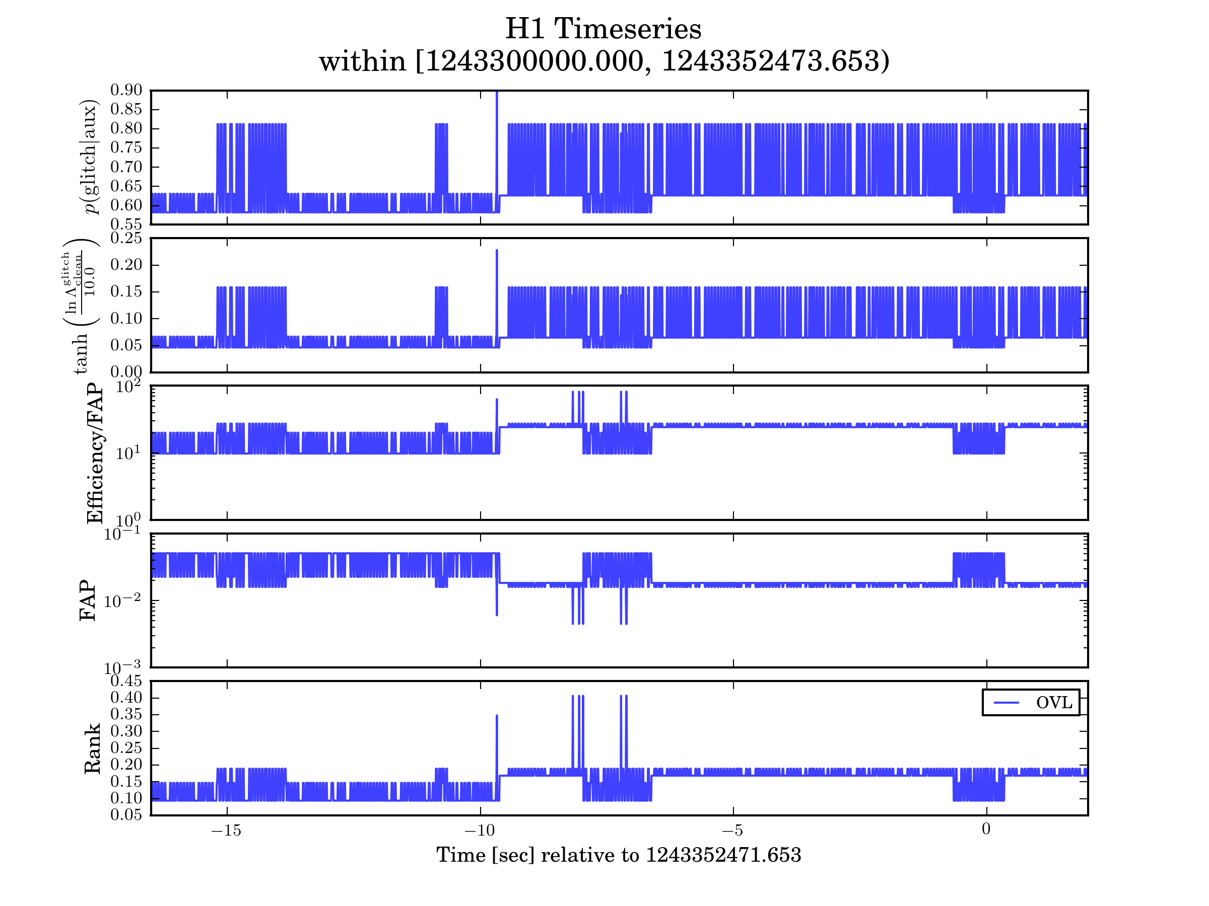
Each panel has a specific meaning related, enumerated below. We note that all these timeseries are inter-related and therefore behavior observed in one will be mirrored in the others. The most fundamental way to see this is to observe that changes in the Rank (bottom panel) produced by the classifier change the rest of the timeseries, as they other timeseries are derived from the Rank.
p(glitch|aux)
The probability that there is a glitch in the target channel (typically a proxy for h(t)) given information about auxiliary channels.
Analysts should interpret this as one might naively expect, with a few important caveats
This probability is calibrated to individual time samples, and therefore searching through a window for any sample above a threshold will introduce an additional trials factor. The mapping between window size and threshold to effective trials factor is not particularly well known, so care must be taken. For example, the probability of seeing p(glitch|aux)>0.9 at any point within a 10 min window is almost surely much larger than 90%.
This probability is computed from the logLikelihood and prior odds. The logLikelihood is informed by the auxiliary channels, but the prior odds measure the relative rate of glitchy and clean samples in iDQ’s evaluation set. Importantly, the rate at which iDQ samples clean times, which is an algorithmic choice unrelated to the physical processes in the detector, can therefore affect the prior odds and p(glitch|aux). This means that, even with an uniformative likelihood, p(glitch|aux) may sit at a non-zero value.
Large values of p(glitch|aux) mean high probability of non-Gaussian noise being present. Please note, this does not necessarily mean the candidate should be rejected, and care must be taken to evaluate whether the non-Gaussian noise witnessed by iDQ could have caused the candidate.
logLikelihood
The likelihood ratio of the auxiliary state of the detector given glitch and clean samples. This is perhaps more fundamentally related to the inference performed by iDQ and does not include the prior odds that are included within p(glitch|aux).
Large values of logLike imply high probability of non-Gaussian noise being present. Please note, this does not necessarily mean the candidate should be rejected, and care must be taken to evaluate whether the non-Gaussian noise witnessed by iDQ could have caused the candidate.
Efficiency/False Alarm Probability
Because iDQ searches for glitches in a target channel using information from auxiliary channels, we can naturally define standard statistical inference quantities, like the detection Efficiency and False Alarm Probability. Many analysts within DetChar estimate the usefulness of a particular veto by the ratio of the Efficiency (fraction of glitches removed) to the False Alarm Probability or Deadtime (fractoin of clean samples removed).
Large values of Eff/FAP correspond to more confident vetoes. If the classifier is behaving reasonably, then this information will be highly degenerate with the classifier Rank and is presented mostly to facilitate comparisons with other glitch detection algorithms.
False Alarm Probability
Estimated as a cumulative integral over p(aux|clean), this represents the probability of accidentally vetoing time that is unassociated with a glitch (the fraction of clean samples removed). This should correspond to the fraction of livetime removed by the veto, assuming the glitch rate is low.
Low FAP values usually correspond to more confident vetoes and higher probability that there is non-Gaussian noise present in the target channel, but this is not always the case. Indeed, the classifier could assign random numbers to samples, producing a poor veto strategy, and still occassionally produce very small FAP. This is why we also report logLike and p(glitch|aux). Therefore, small FAPs do not necessarily mean the candidate should be rejected, just that hte auxiliary state is relatively rare.
Nonetheless, the FAP provides a useful way to define the working point, in that it defines the amount of livetime one is willing to sacrafice when vetoing noise. Please note, searching through a window for any sample with FAP below a threshold will introduce an additional trials factor. That mapping is not particularly well known, so the actual amount of time vetoed based on such a strategy will not correspond to the threshold place on FAP. Indeed, the probability of seeing FAP < 0.1 in 100 sec is quite high, and therefore the deadtime induced by throwing out anything with FAP < 0.1 within 100 sec will be much larger than 10%.
Rank
This is the most fundamental statistic produced by iDQ’s trained classifiers, but also is the least interpretable. Classifiers act to reduce the high-dimensional auxiliary state into a single scalar (Rank), attempting to map glitchy states to near Rank=1 and clean states near Rank=0. However, the precise value of Rank has no intrinsic meaning. This is why iDQ calibrates its output into probabilistic measures, like logLike.
Large values of Rank do imply the classifier believes there is non-Gaussian noise present, but this does not necessarily mean the candidate should be rejected. Care must be taken to evaluate the statistical significance of that value of Rank (e.g., FAP or p(glitch|aux)) and to determine whether the non-Gaussian noise could have caused the candidate.
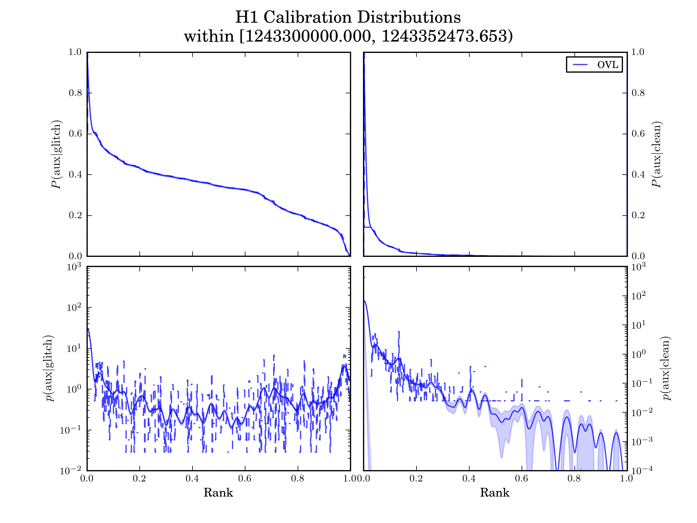
Calibration Distributions
iDQ calibrates the output of each classifier (Rank) into several probabilistic quantities. This is done by directly measuring the conditioned likelihoods over rank. The Calibration Distributions are shown for reference in figures like the following. If there is a lot of variability in the calibration distributions (i.e., multiple curves on each panel that do not agree), this may indicate that iDQ’s calibrations are not accurate and therefore iDQ information may not be reliable. However, this is not expected to occur frequently.
Feature Importance
Supervised learning algorithms within iDQ may be able to identify measures of the relative importance of different auxiliary features. These can be presented as a figure and/or a table. Please note, not all algorithms currently provide measures of feature importance, and therefore this information may or may not be present depending on how iDQ is configured.
OVL’s Feature Importance Figure and Tables
A common (benchmark) algorithm run under iDQ is OVL. OVL provides intutive notions of feature importance as it applies separare veto conditions based on single auxiliary channels in a hierarchical order, with the configurations applied first naturally believed to be the most important. This information is presented in both a figure and table, and examples are shown below.
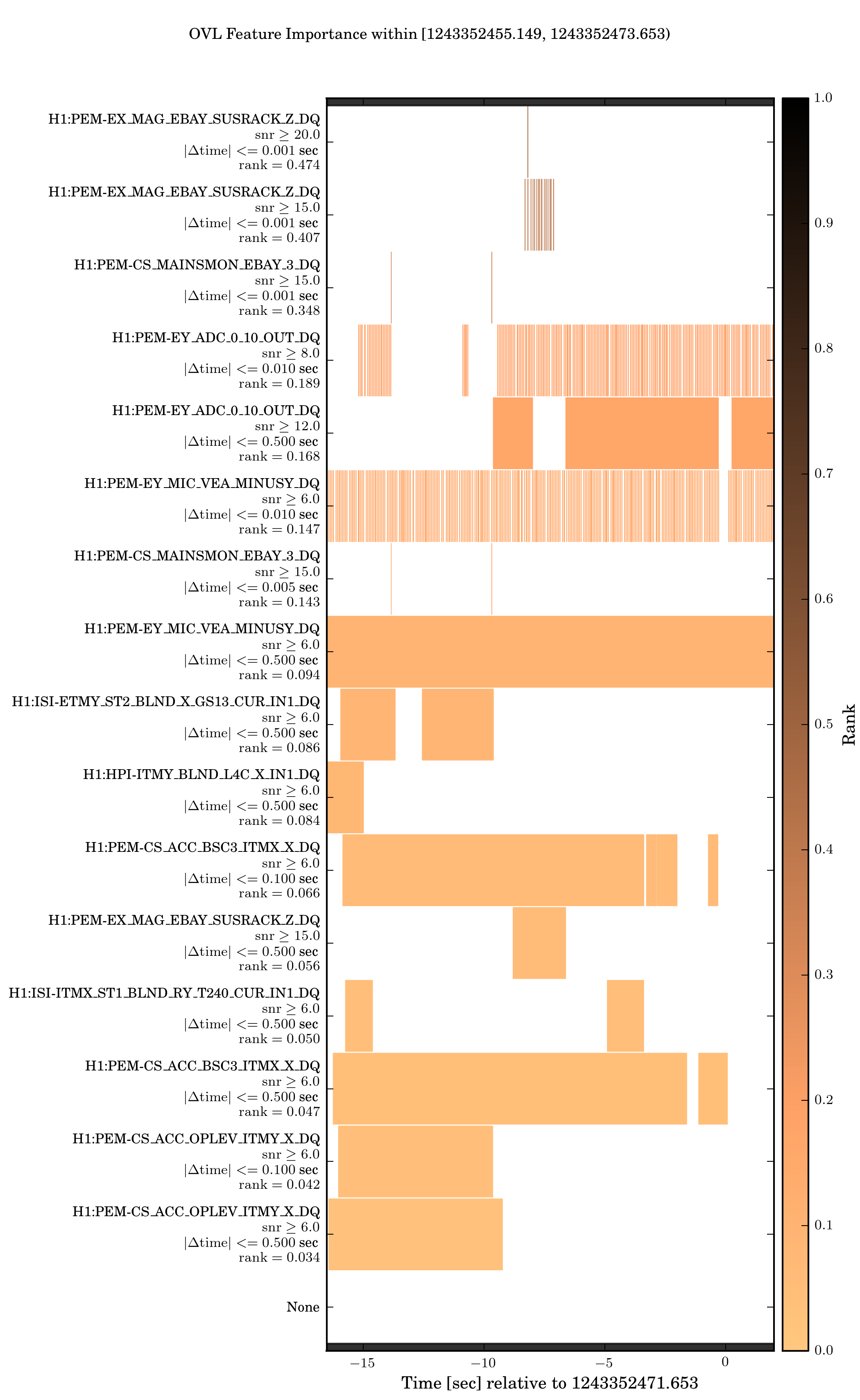
OVL’s feature importance figures show which auxiliary configurations were active during this time period, with colors indicating the Rank associated with each configuration. This is the same Rank reported in the timeseries figures, which is calibrated via the Calibration Distributions into probabilistic measures. Each configuration is labeled by the auxiliary channel, a threshold on glitches’ amplitude in the the auxiliary channel, a time window, as well as the numerical value of the Rank. Configurations with bigger Ranks are applied first and show up at the top of this figure.
If analysist observe excursions in the timeseries, they may refer to these plots to immediately determine which auxiliary witness is associated with the excursion. Anectdotal evidence often suggests the source of noise and its morphology in the target channel based on which auxiliary channels witnessed it.
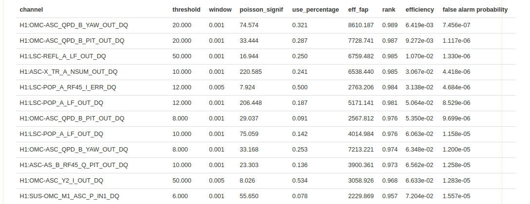
OVL also presents the full Vetolist associated with the classifier. This allows analysts to see which channels were believed to be correlated with noise in the target channel at that time. Analysts may wish to refer to this list to determine the types of noise witnessed. For example, if the are no excursions in the timeseries surrounding the event, the conclusion may be very different if OVL found many different auxiliary witnesses for noise (a long Vetolist) and none of them were active compared to cases where OVL simply couldn’t find many witnesses for noise (a short Vetolist) and therefore nothing was active.
For each veto configuration in the Vetolist, we report the
auxiliary channel
threshold on amplitude in the auxiliary channel (only active if there is a glitch above this threshold in the aux channel)
window surrounding glitches in the aux channel over which the veto condition is active
poisson_signif
an incremental measure of the probability that a veto condition would be coincident with glitches in the target channel due to pure chance.
larger values of poisson_signif imply lower probability of chance coincidence
use_percentage
an incremental measure of the fraction of times the veto condition vetoed a glitch when it was active
larger values of use_percentage imply more deterministic auxiliary witnesses
eff_fap (Efficiency/FAP)
an incremental estimate of the efficiency and FAP associated with each veto condition
larger values of eff_fap imply more effective auxiliary witnesses.
rank
cumulative Efficiency determined by applying the Vetolist in order during training
cumulative FAP determined by applying the Vetolist in order during training
Within the Full iDQ Summary Report
The full iDQ summary report, which is only available in high-latency (~hours) and will be linked from the DQR, contains all the information rendered within the DQR HTML interface and more. We briefly describe the additional information availble below.
Analysts should expect to navigate around the full iDQ summary pages to find both comparisons between multiple classifiers and single-classifier results. This provides a deep-dive into the types of correlations witnessed by iDQ and their ability to identify noise in the target channel.
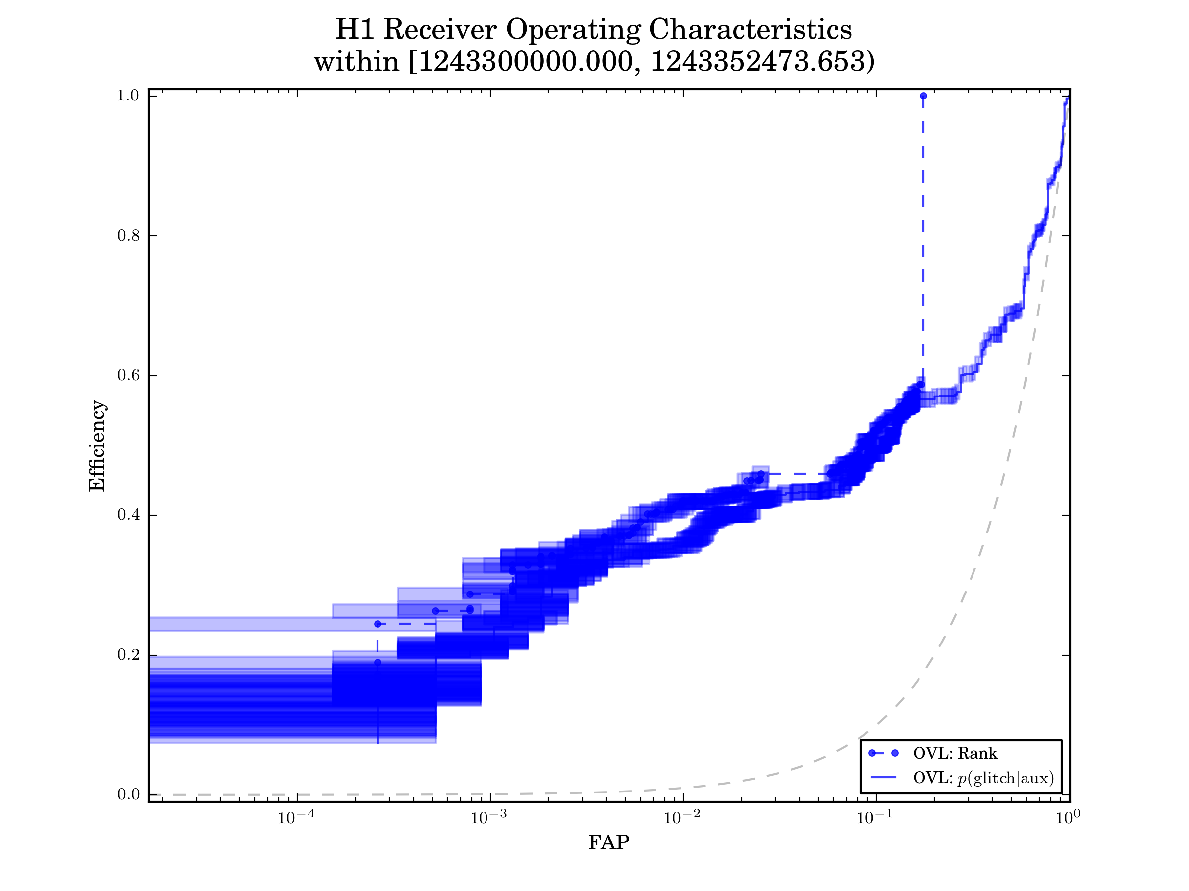
Receiver Operating Characteristic Curves
Using data from a broader window than the small query presented in the DQR HTML interface, iDQ estimates the Receiver Operating Characteristic (ROC) curve for each classifier around the event. This requires a broad window because we are limitted by sample statistics (narrow window implies few samples). There are 2 ROC curves presented for each classifier
Rank
we estimate the ROC curve by ordering samples by the rank assigned by the classifier. If multiple models were used to rank the samples within the broad window (i.e., the asynchronous training jobs updated the model), then these ranks may not have the same intrinsic meaning. However, they should demonstrate something like the underlying performance expected for each classifier.
p(glitch|aux)
we estimate the ROC curve by interpolating the p(glitch|aux) timeseries to assign a value to each sample, and then order according to that. If the classifiers and calibration are behaving well, we expect this estimate to closely follow the estimate using Ranks. Typically, if the p(glitch|aux) ROC curve falls below the Rank ROC curve, this indicates that the calibration is struggling to accurately describe the conditioned likelihoods produced by the classifier.
An example is shown below. This is fairly typical performance for OVL (ranking metric=eff_fap) using GSTLAL features.
Calibration Coverage
iDQ’s calibration depends on the ability to accurately measure the conditioned likelihoods associated with each classifier. We in turn estimate this by checking the coverage for the cumulative distributions of each likelihood. That is to say, we expect X% of glitches to be assigned an Efficiency below X% for any value of X. Calibration coverage plots, like the following, estimate this by interpolating the timeseries to assign Efficiency and FAP values to each sample and then constructing cumulative distributions. Error bars represent ~1-sigma uncertainty from counting statistics; we only have a finite number of samples. If the pipeline is properly calibrated, then the nominal fraction of samples should match the observed fraction of samples, and we should see diagonal curves like the following.
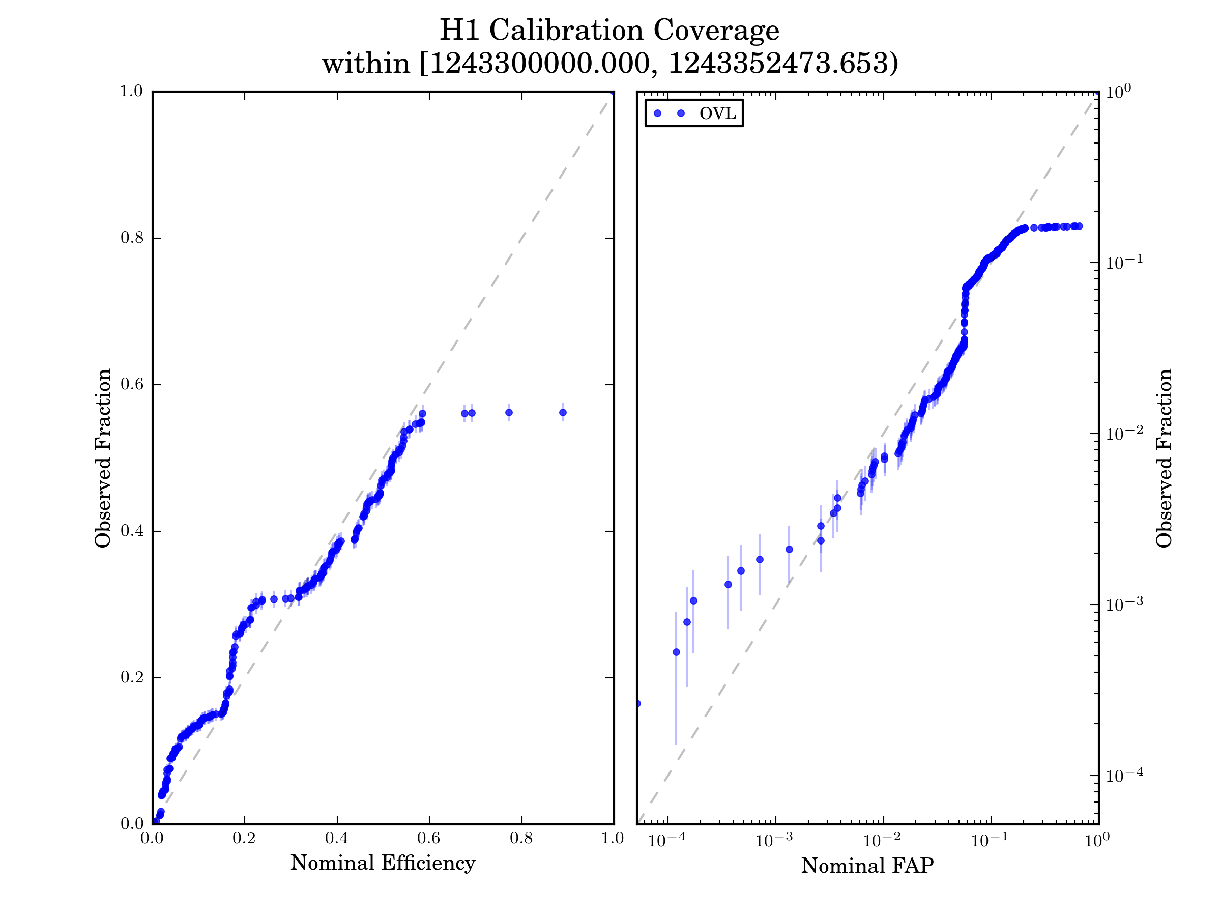
We note that the calibration coverage mostly follows the diagonal line, but occassionally deviates more than the sample uncertainty would suggest. This is believed to be associated with 2 causes
non-stationarity in the detectors can change the conditioned likelihoods faster than the asynchronous calibration job can respond at times. This can produce off-diagonal behavior
interpolation artifacts and oversmoothing inherent in the representation of the conditioned distributions can produce step-like off-diagonal behavior. An example of this can be seen at high FAP in the above figure. Because many clean samples are assigned Rank=0, the Gaussian Kernel Density Estimate (KDE) used to represent the conditioned likelihood will assign some weight to Ranks slightly larger than 0. This is apparent in the p(aux|clean) distribution shown below.
This means that the nominal FAP will be larger than the true FAP (tthe cumulative distribution picks up the KDE’s tail) until we reach Rank=0, at which point the observed FAP will jump up to match the nominal value. This can occur at any Rank, and can be associated with first over-coverage (nominal fraction > observed fraction) and then under-coverage (nominal fraction < observed fraction).
These figures show typical calibration performance for OVL using GSTLAL features, and analysts should not be concerned unless they see significantly larger deviations from the diagonal than what are shown here.
Single-Classifier Deep-Dives
The full summary reports also contain detaild breakdowns of each classifier’s performance, including estimates of the calibration coverage and distributions for each CalibrationMap used within the wide window as well as estimates of the ROC curves and feature importance for each ClassifierModel used. Again, because the iDQ online jobs only report the results of independent, asynchronous processes managed outside the DQR, there may be multiple CalibrationMaps and ClassifierModels used to generate timeseries within any time window.
Analysts are unlikely to need this level of detail. However, if they observe poor calibration coverage or ROC curves in the agglomerated summary plots, they may wish to search through the individual behavior of each CalibrationMap and ClassifierModel to determine whether this is due to a systematic (long-lived) issue or is associated with only a single Map or Model.
What INI options, config files are required?
config (string)
a path to a config file
nicknames (string)
a space-delimited list of nicknames that should be included in the report to GraceDb
delay (float, optional)
the number of seconds to wait before querying data. This allows us to reasonably guarantee that data is discoverable through standard tools (gw_data_find).
Are there any derived tasks that are based on this one?
The following reference standard iDQ configs stored within the DQR source code and therefore will ignore config if it is supplied.
H1 iDQ online
L1 iDQ online
H1 iDQ online-kw
L1 iDQ online-kw