Sample release
This notebook serves as a basic introduction to loading and viewing data released in associaton with the publication titled GW190814: Gravitational Waves from the Coalescence of a 23 Msun Black Hole with a 2.6 Msun Compact Object.
The released data file can be read in using the PESummary or h5py libraries. For general instructions on how to manipulate the data file and/or read this data file with h5py, see the PESummary docs
First we import the key python modules
[1]:
%matplotlib inline
import pesummary
from pesummary.io import read
print(pesummary.__version__)
/usr/local/lib/python3.10/site-packages/gwpy/time/__init__.py:36: UserWarning: Wswiglal-redir-stdio:

SWIGLAL standard output/error redirection is enabled in IPython.
This may lead to performance penalties. To disable locally, use:

with lal.no_swig_redirect_standard_output_error():
    ...

To disable globally, use:

lal.swig_redirect_standard_output_error(False)

Note however that this will likely lead to error messages from
LAL functions being either misdirected or lost when called from
Jupyter notebooks.

To suppress this warning, use:

import warnings
warnings.filterwarnings("ignore", "Wswiglal-redir-stdio")
import lal

  from lal import LIGOTimeGPS
1.6.2.dev24+g52b59f12f
As part of this sample release, we are releasing the posterior samples generated from 15 different analyses. The samples for each analysis is stored in the data file. This data file can be read in using the ‘pesummary’ read function
[2]:
file_name = 'GW190814.h5'
data = read(file_name)
2026-04-01  22:55:30 PESummary WARNING : Could not find f_final in input file and one was not passed from the command line. Using 1024.0Hz as default
2026-04-01  22:55:30 PESummary WARNING : Could not find delta_f in input file and one was not passed from the command line. Using 0.00390625Hz as default
2026-04-01  22:55:30 PESummary WARNING : Could not find f_start in input file and one was not passed from the command line. Using 20.0Hz as default
2026-04-01  22:57:13 PESummary WARNING : Could not find f_final in input file and one was not passed from the command line. Using 1024.0Hz as default
2026-04-01  22:57:13 PESummary WARNING : Could not find delta_f in input file and one was not passed from the command line. Using 0.00390625Hz as default
2026-04-01  22:57:13 PESummary WARNING : Could not find f_start in input file and one was not passed from the command line. Using 20.0Hz as default
The posterior samples can be extracted through the samples_dict property. These posterior samples are stored in a custom table structure
[3]:
samples_dict = data.samples_dict
posterior_samples = samples_dict['combined']
parameters = list(posterior_samples.keys())
print(parameters)
['recalib_L1_frequency_6', 'recalib_V1_phase_2', 'V1_matched_filter_abs_snr', 'recalib_H1_phase_2', 'recalib_V1_amplitude_0', 'log_likelihood', 'recalib_L1_phase_1', 'recalib_V1_phase_9', 'recalib_H1_frequency_7', 'recalib_L1_frequency_2', 'recalib_V1_amplitude_8', 'recalib_H1_amplitude_0', 'recalib_H1_frequency_2', 'recalib_L1_phase_5', 'spin_1y', 'V1_matched_filter_snr_angle', 'peak_luminosity', 'recalib_L1_frequency_0', 'final_spin', 'recalib_H1_frequency_5', 'V1_optimal_snr', 'recalib_L1_amplitude_2', 'psi', 'phi_2', 'chi_2_in_plane', 'recalib_V1_frequency_3', 'recalib_H1_frequency_9', 'recalib_V1_phase_0', 'recalib_H1_phase_8', 'recalib_H1_frequency_4', 'recalib_V1_amplitude_1', 'recalib_V1_phase_5', 'recalib_V1_phase_7', 'spin_1z', 'recalib_H1_phase_0', 'recalib_H1_amplitude_4', 'mass_2', 'recalib_L1_amplitude_3', 'recalib_H1_phase_4', 'chi_eff', 'H1_time', 'spin_1x', 'cos_iota', 'recalib_L1_phase_6', 'recalib_L1_frequency_1', 'recalib_L1_phase_2', 'time_jitter', 'recalib_V1_amplitude_9', 'L1_optimal_snr', 'recalib_V1_frequency_7', 'spin_2y', 'V1_time', 'recalib_H1_frequency_0', 'recalib_L1_amplitude_7', 'recalib_V1_frequency_8', 'recalib_H1_amplitude_6', 'recalib_H1_frequency_6', 'recalib_L1_phase_3', 'recalib_V1_frequency_4', 'mass_ratio', 'recalib_H1_amplitude_2', 'phi_jl', 'recalib_V1_amplitude_5', 'H1_matched_filter_snr_angle', 'L1_matched_filter_snr', 'recalib_H1_amplitude_7', 'recalib_V1_amplitude_4', 'tilt_2', 'recalib_L1_frequency_3', 'recalib_H1_frequency_1', 'recalib_L1_frequency_4', 'phase', 'symmetric_mass_ratio', 'L1_matched_filter_abs_snr', 'cos_tilt_2', 'phi_1', 'cos_theta_jn', 'geocent_time', 'recalib_V1_amplitude_7', 'iota', 'recalib_H1_phase_5', 'recalib_H1_frequency_3', 'chi_1_in_plane', 'H1_matched_filter_snr', 'recalib_L1_frequency_5', 'recalib_L1_frequency_9', 'recalib_L1_amplitude_6', 'recalib_L1_phase_7', 'recalib_H1_phase_7', 'recalib_L1_frequency_8', 'theta_jn', 'dec', 'recalib_V1_phase_8', 'L1_matched_filter_snr_angle', 'H1_optimal_snr', 'recalib_V1_frequency_2', 'recalib_H1_amplitude_5', 'chi_p', 'L1_time', 'recalib_V1_phase_1', 'recalib_H1_amplitude_3', 'recalib_L1_amplitude_1', 'spin_2z', 'ra', 'H1_matched_filter_abs_snr', 'recalib_H1_amplitude_9', 'recalib_V1_phase_3', 'spin_2x', 'cos_tilt_1', 'recalib_L1_amplitude_4', 'recalib_V1_frequency_9', 'recalib_H1_phase_3', 'recalib_L1_phase_9', 'recalib_L1_frequency_7', 'inverted_mass_ratio', 'recalib_L1_phase_8', 'phi_12', 'a_2', 'recalib_H1_phase_6', 'chirp_mass', 'recalib_L1_amplitude_8', 'recalib_V1_frequency_6', 'recalib_V1_phase_6', 'luminosity_distance', 'final_mass', 'tilt_1', 'mass_1', 'recalib_V1_amplitude_2', 'recalib_V1_amplitude_3', 'recalib_V1_amplitude_6', 'recalib_L1_amplitude_0', 'total_mass', 'recalib_V1_frequency_1', 'recalib_H1_phase_9', 'recalib_L1_amplitude_9', 'recalib_V1_frequency_5', 'recalib_H1_phase_1', 'a_1', 'recalib_H1_amplitude_8', 'recalib_H1_frequency_8', 'recalib_L1_phase_0', 'recalib_V1_phase_4', 'comoving_distance', 'recalib_V1_frequency_0', 'recalib_L1_amplitude_5', 'network_optimal_snr', 'recalib_H1_amplitude_1', 'recalib_L1_phase_4', 'V1_matched_filter_snr', 'redshift', 'mass_1_source', 'mass_2_source', 'total_mass_source', 'chirp_mass_source', 'final_mass_source', 'radiated_energy', 'network_matched_filter_snr']
combined analysis
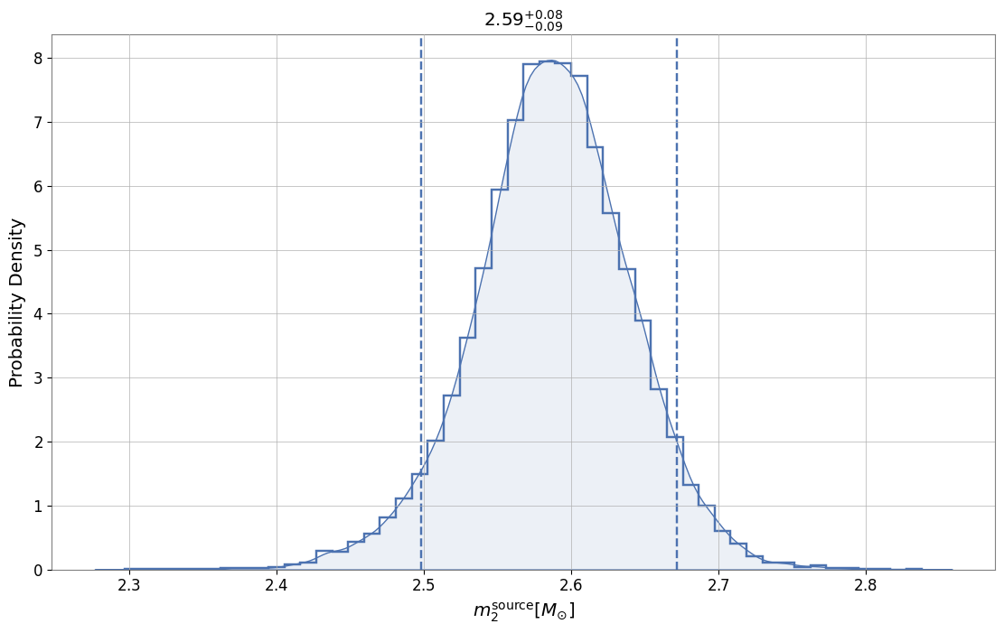
‘pesummary’ allows for the user to easily make plots. As an example, we show the posterior distribution for ‘mass_2_source’ plotted as a KDE.
[4]:
fig = posterior_samples.plot('mass_2_source', type='hist', kde=True)
fig.set_size_inches(12, 8)
fig.show()
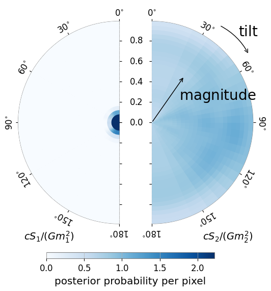
We may also easily generate a spin disk, showing the most probable direction of the spin vectors
[5]:
fig = posterior_samples.plot(type='spin_disk', colorbar=True, annotate=True, show_label=True, cmap='Blues')
fig.show()
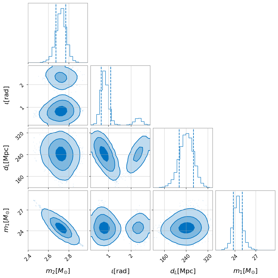
Corner plots are very useful for spotting degeneracies between parameters. A corner plot can easily be generated using ‘pesummary’
[6]:
fig = posterior_samples.plot(type='corner', parameters=['mass_1', 'mass_2', 'luminosity_distance', 'iota'])
fig.show()
Comparing multiple analyses
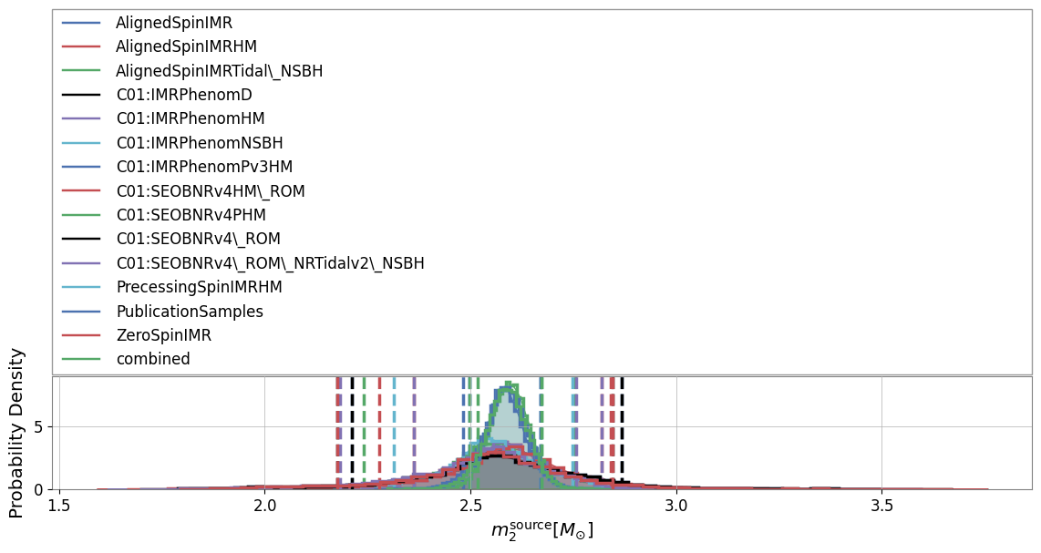
As the ‘pesummary’ file is able to store multiple analyses in a single file, we are able to easily generate a comparison plot showing the posterior distribution for ‘mass_2_source’ for each analysis
[7]:
fig = samples_dict.plot('mass_2_source', type='hist', kde=True)
fig.set_size_inches(12, 8)
fig.show()
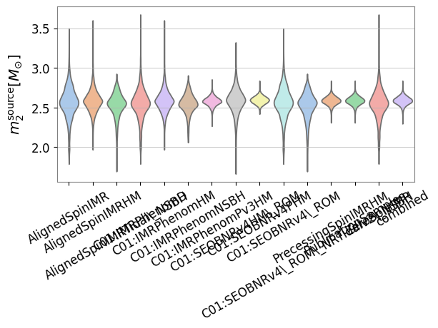
A comparison histogram is not the only way to display this data. We may also generate a violin plot showing the posterior distribution for each analysis
[8]:
fig = samples_dict.plot('mass_2_source', type='violin')
fig.show()
/usr/local/lib/python3.10/site-packages/pesummary/core/plots/seaborn/violin.py:137: FutureWarning:

The `scale` parameter has been renamed and will be removed in v0.15.0. Pass `density_norm='width'` for the same effect.
  return categorical.violinplot(*args, **kwargs)
/usr/local/lib/python3.10/site-packages/pesummary/gw/plots/publication.py:241: UserWarning: set_ticklabels() should only be used with a fixed number of ticks, i.e. after set_ticks() or using a FixedLocator.
  ax1.set_xticklabels(labels)
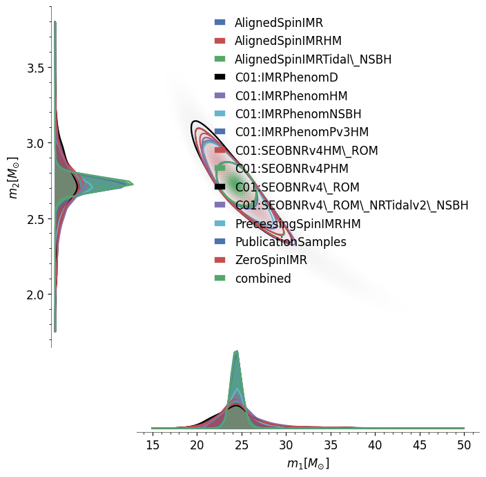
‘pesummary’ also allows for the user to generate a triangle plot with ease
[9]:
fig = samples_dict.plot(['mass_1', 'mass_2'], type='reverse_triangle', grid=False)
fig[0].show()
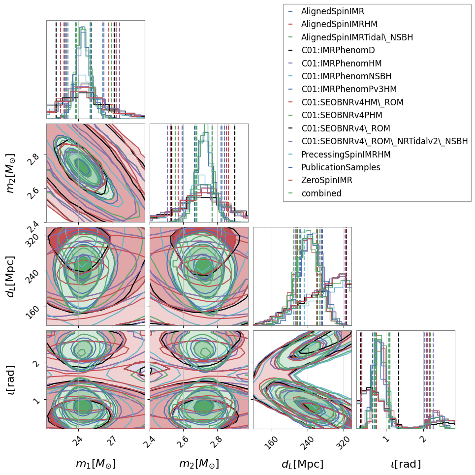
It is also useful to see how degeneracies between certain parameters change for different analysis. This can be investigated by generating a comparison corner plot
[10]:
fig = samples_dict.plot(type='corner', parameters=['mass_1', 'mass_2', 'luminosity_distance', 'iota'])
fig.show()
PSD data
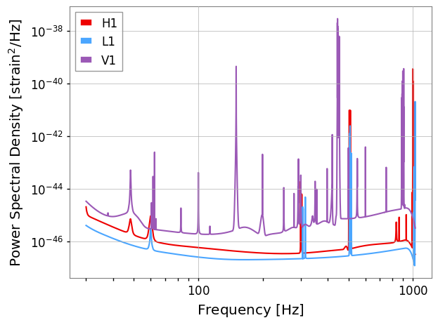
The ‘pesummary’ file also stores the PSD that was used for each analysis. This can be extracted and plotted
[11]:
psd = data.psd['combined']
fig = psd.plot(fmin=30)
fig.show()
