Hyper-parameters

This short guide will illustrate how to estimate hyper-parameters from posterior samples using bilby using a simplistic problem.

Setting up the problem

We are given three data sets labelled by a, b, and c. Each data set consists of $N$ observations of a variable $y$ taken at a dependent variable $x$. Notationally, we can write these three data sets as $(y_i^a,x_i^a),(y_i^b,x_i^b),(y_i^c,x_i^c)$ where $i\in [0,N]$ labels the indexes of each data set.

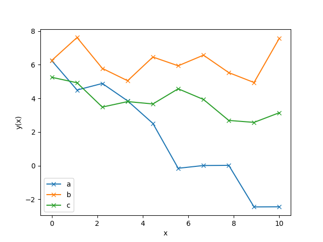
Plotting the data, we see that all three look like they could be modelled by a linear function with some slope and some intercept:

Given any individual data set, you could write down a linear model $y(x)=c_0+c_{1}x$ and infer the intercept and gradient. For example, given the a-data set, you could calculate $P(c_0|y_i^a,x_i^a)$ by fitting the model to the data. Here is a figure demonstrating the posteriors on the intercept, for the three data sets given above

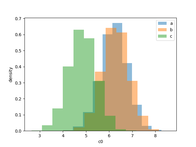
While the data looks noise, the overlap in the $c_0$ posteriors might (especially given context about how the data was produced and the physical setting) make you believe all data sets share a common intercept. How would you go about estimating this? You could just take the mean of the means of the posterior and that would give you a pretty good estimate. However, we’ll now discuss how to do this with hyper parameters.

Understanding the population using hyperparameters

We first need to define our hyperparameterized model. In this case, it is as simple as

$$c_0\sim \mathcal{N}({\mu }_{c_0},{\sigma }_{c_0})$$

That is, we model the population $c_0$ (from which each of the data sets was drawn) as coming from a normal distribution with some mean and some standard deviation.

To do - write in details of the likelihood and its derivation

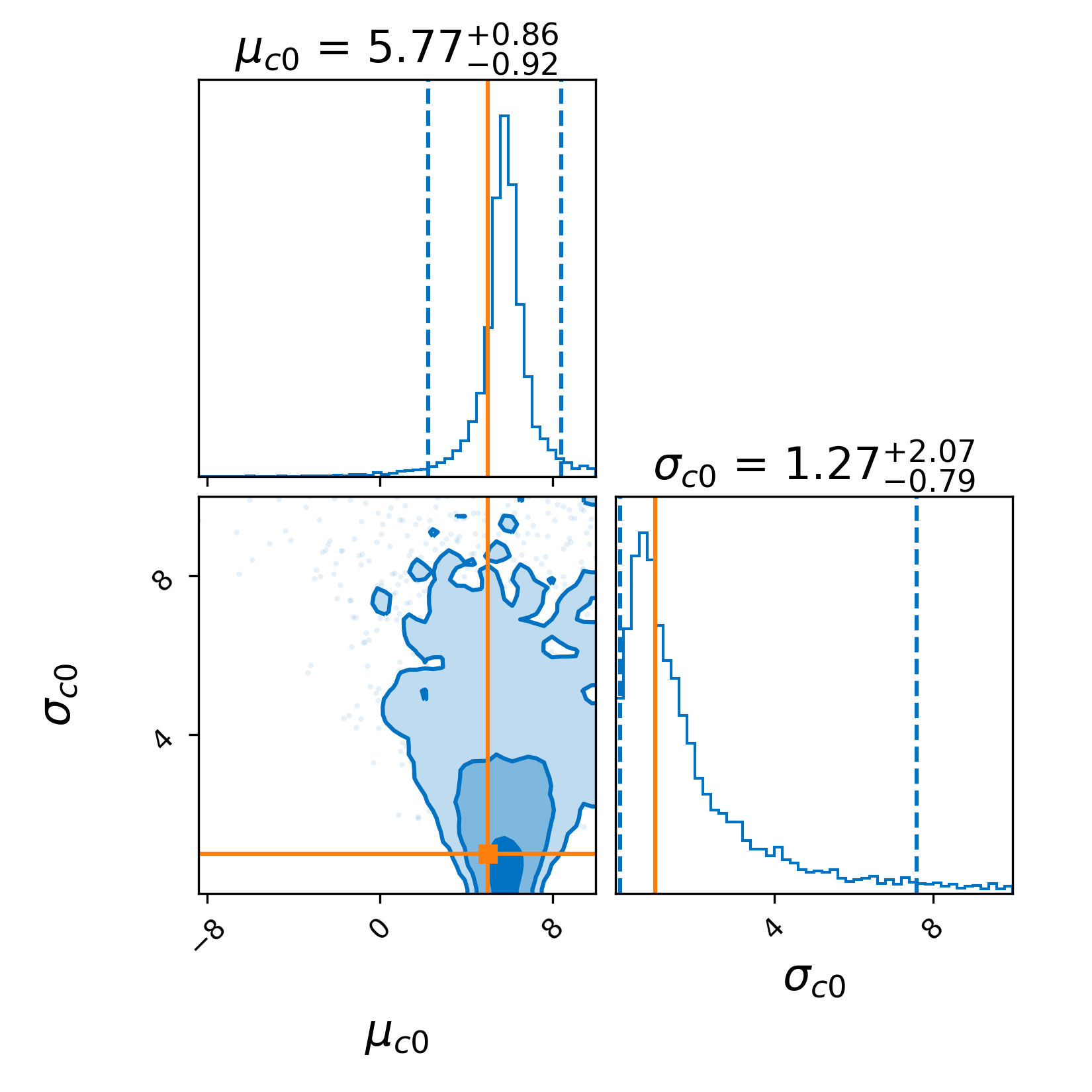
For the samples in the figure above, the posterior on these hyperparamters is given by